Particle Filter Based
Fast Simultaneous Localization and Mapping
Utku Çulha#1, Bilal Turan#2
#Computer Engineering Department, Bilkent University
Bilkent, 06800, ANKARA, TURKEY
Abstract— With respect to the necessity of more autonomous capabilities for mobile robotics in ubiquitous terrains, capable methods on localization and mapping have been developed for the last decade. One of these methods is the Fast SLAM approach which is an extension of the original SLAM problem suggested.
In this report we are expressing our methodology for applying a Fast SLAM method based on particle filters applied on the generating map. Differing from its continuous space relatives, in particle filter based Fast SLAM we are considering discrete samples in the robot world covering map poses, sensor and motion models.
In our experiments we have used a simulation platform consisting of 3 different map types for a mobile robot existing in a 2D world.
Keywords— Fast SLAM, Particle Filters, Sensor Model
I. INTRODUCTION
The problem for autonomous localization and mapping for mobile robots is one of the most fundamental topics researches are interested in. The main problem in this topic is that the robot’s pose and the map is unknown at the same time, therefore probabilistic approaches upon this problem depends on the information coming from the user commands and the sensor readings from the range devices on the robot.
The general name given for this kind of approach is simultaneous localization and mapping or SLAM in short.[1] In this approach the main aim is to estimate the posterior pose of the robot and the map surrounding it with respect to the user controls and sensor readings. This aim can be defined as:
![]() (1)
(1)
Where x denotes the pose of the robot (pose of the robot changes with respect to the problem space; it consists of 6 variables if the space is 3D and 3 variables as x, y and θ for 2D environments), m denotes the map. The given probabilities z is the sensor reading and u is the control command. In the Equation 1 the posterior pose of the robot is estimated for the time stance t, which is one of SLAM’s different applications. In this case only the current pose of the robot and the map around it is estimated with given inputs which is called online SLAM.[1]-[4] For the Full SLAM case, this posterior is estimated for the total of time stances, in other words, starting from time 1 to t.
A naive implementation of Fast SLAM algorithm is doomed to fail because of the dimensionality problem. Here if we are going to use this formula as it is, meaning if we see the map and the position is dependent to each other, our state dimension becomes very large and hence the problem becomes infeasible.
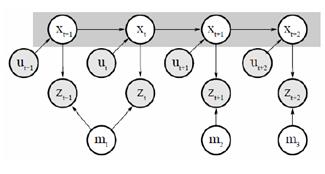
Fig. 1 Bayes network for the Fast SLAM problem
If we knew the history of robot poses, then map features will become independent. This greatly simplifies equation 1 into:
![]()
![]() (2)
(2)
Equation 2 can be simplified even further if we use the main property of the grid maps. In grid maps every individual cell is independent from each other. Thus equation 2 further simplifies into:
![]()
![]() (3)
(3)
All this assumptions and simplifications make the Fast SLAM algorithm feasible. Still there are many issues that must be solved in Fast SLAM and surely one must do some clever implementation to be able to have a real time Fast SLAM.
II. FAST SLAM ALGORITHM
We have simplified the Fast SLAM problem and get the equation 3 with some clever assumptions. After stating the independence of the pose of the robot and landmarks in the environment, the problem becomes more implementable.
We can use a Particle Filter to estimate the robot pose at any time, then we will use separate Gaussian Filters to estimate different landmarks.
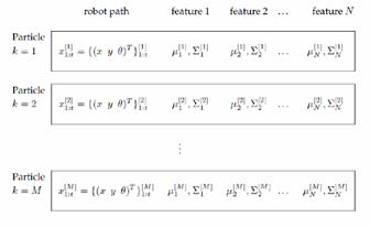
Fig. 2 Rao-Blackwellized particle filtering based on landmarks [2]
As in the Figure 2, As Rao-Blackwellized suggest we can have an implementable particle based Fast SLAM algorithm. Here every landmark represented by a 2D EKF and we have M different particles for robot pose.
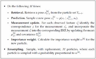
Fig. 3 A simple pseudo code for Fast SLAM
Figure 3 shows a simple pseudo code for Fast SLAM algorithm, using EKF for a landmark based mapping. First question that arise in this implementation is how to find correspondences between measurements and the landmarks in the environment. If we do not have unique landmarks we might have different combination of correspondences. If we have used an EKF Filter for robot pose, then wrong data associations might cause filter to diverge. But luckily in Particle Filter implementation since we have different particles meaning different robot poses, we have different data associations for different particles. Hence even if we have wrong data association for a particle only that particle will become less probable in succeeding data measurements and the main algorithm will not fall apart easily.
poses are known the Occupancy Grid Mapping is easy. Each particle has its own map. Hence the problem with Occupancy Grid Mapping is since we have 2D grids for the environment space and computational requirement for the algorithm is enormous. Therefore we must keep the particle number small in order to have a feasible implementation.
Pseudo code in Figure 3 does not change much for Occupancy Grid Mapping. The only change is at measurement update part, now we have 2D grid map instead of landmarks. For prediction part we need to implement a motion model, for importance weight we have to implement a sensor model and as for measurement update we need to have the inverse of the sensor model we have implemented. Resampling and retrieval part is simple and hence does not require any detailed explanation.
III. MOTION MODEL
The motion model in the Fast SLAM approach basically forms the particles estimated in each movement of the robot. This movement is dependent on the noisy motion commands which are assumed to be given in the whole posterior probability model.
As Fast SLAM is applied on particle based filters, the motion model in the approach is a discrete sampling method which creates distinct pose estimates given the motion commands and its resulting actions. With respect to our experiments in the simulations, our motion model is compliant with the 2D world motion rules and variables. The general motion in this world can be explained with the figure below.
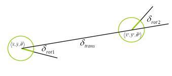
Fig. 4 The motion model in 2D world
The figure above shows a single motion built up with 3 consequent action sub-forms, δrot1, δtrans and δrot2. These sub-forms are calculated by using the state variables of the initial and final robot poses. One important fact here is that these poses are found by using the encoders of the robot which generally produces noisy data. The motion model of the whole approach includes this sensor noise which is called also as the command noise. These sub-forms are calculated as below:
![]() (4)
(4)
![]() (5)
(5)
![]() (6)
(6)
In order to model the sensor noise in the motion model, a sample function of the Gaussian is applied on these sub-forms. The noise model applied is as follows:
![]() (7)
(7)
![]() (8)
(8)
![]() (9)
(9)
These noise models include the Gaussian distribution samples from the noisy encoder data on each iteration of robot motion. By using these forms the general motion model is derived. This derivation can be seen in a pseudo format in the following figure.
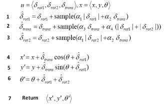
Fig. 5 Algorithm for motion model
It can be seen that the result of the motion model is a pose estimate based on the calculations done on the noisy odometry data coming from encoders. In order to generate a particular number of particles, in other words pose estimates, the algorithm above is executed several times on the same odometry data.
IV. SENSOR MODEL
Sensor model gets the known robot pose from a particle and gets reading data from Sick Laser of the robot, using the interface of the Aria. From Sick Laser we get 180 different laser readings each representing a different degree. For sensor model we find probability of a given measurement and pose according to these readings. These values are used as importance weight in our algorithm. Here we assume the map is known, at least the part of it which is mapped so far. We are using a simple threshold for finding obstacles in our map. Equation 4 and 5 shows derivation of sensor model.
![]() (10)
(10)
Using the assumption that different rays are independent of each other:
![]() (11)
(11)
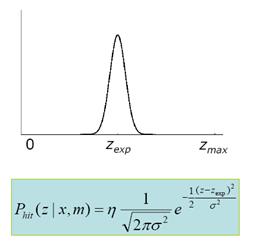
Fig. 6 Gaussian model for ray casting method
We actually simplified sensor model a bit. We ignore the max readings and some readings that are too short. This improves our algorithms performance. Apart from that we are using Gaussian model in the above figure. More generic algorithm is below:
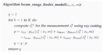
Fig. 7 Algorithm for sensor model
Inverse sensor model is quite different than this. Actually we have used the cone model, but since we have a Sick Laser and 180 different measurements, our cone model become a ray model, but underlying assumptions is just same.
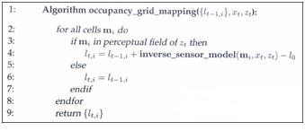
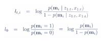
Fig. 8 Algorithm for adding new measurements into map
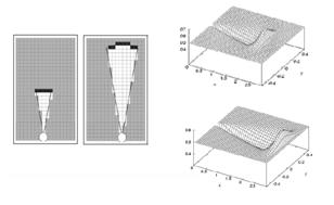
Fig. 9 Illustration of Cone model for implementing inverse sensor model
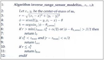
Fig. 10 Algorithm of Cone model for implementing inverse sensor model
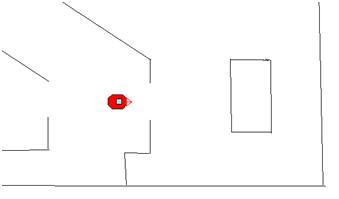
Fig. 11 A sample pose and map from MobileSim
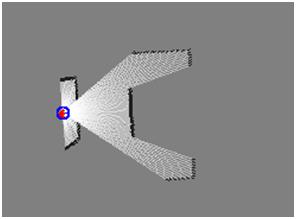
Fig. 12 Inverse sensor model for of the above figure
V. IMPORTANCE WEIGHT
For every particle, given the latest range sensor data, we find probabilities to use in resampling process. Using probabilities directly is not a good way to start since generally probabilities differ in orders of ten. So we take logarithm of the probabilities. Then we normalize them by making the minimum non-infinity probability zero. From that point the probability of a particle to be chosen for resampling is proportional with its weight. This is the main point of the algorithm which makes it robust to the noises.
VI. EXPERIMENTS
In order to see the result of the Fast SLAM algorithm based on particle filters, we have used the simulation environment of Aria which is provided by MobileSim.[5] This simulator enabled us to control a p3dx robot with 2 wheel encoders, range sonars and a SICK laser.
We have created 3 different maps using the Mapper3 software. Each of these maps consists of different level of paths for the robot. We have tried to create narrow corridors and broad halls in order to harden the Fast SLAM problem. What is more, beyond using particles in the map we have adopted the grid base map scheduling with grid sizes 50 pixels in a 1000x1000 pixel maps. In order to visualize the simultaneously generated map we have used an open source library OpenCV[6].
In order to implement a full autonomous Fast SLAM algorithm, we have also applied an exploration method for our robot. In this method, the robot wanders the unexplored areas in the map and generates the maps via the approach of Fast SLAM. Through this exploration, our motion model generates 15 particles in each iteration of robot motion. These particles are then re-sampled with respect to the weights computed in order to correct the noisy maps and ignore falsely estimated poses.
We have run our models in a Dual-Core Pentium 2.0 GHz machines to improve the computation capability.
VII. RESULTS
Below are the results depending on the experiment run on the first map:
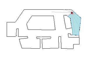
Fig. 13 Our first map in MobileSim environment
The images below show the SLAM results generated every 20 steps covered in the algorithm. The result images start with a map of grids having 0.5 probabilities. While algorithm evolves the grid map converges to the real map shown above.
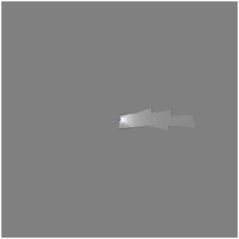
Fig. 14 Map generated at the beginning of the algorithm
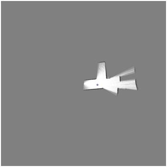
Fig. 15 Map generated at the later steps of the algorithm
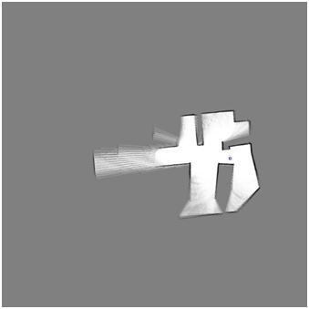
Fig. 16 Map generated at the later steps of the algorithm
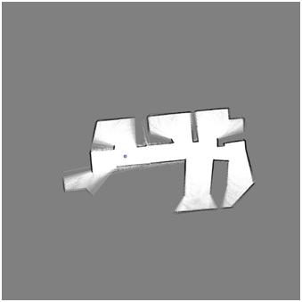
Fig. 17 Map generated at the later steps of the algorithm

Fig. 18 Map generated at the later steps of the algorithm
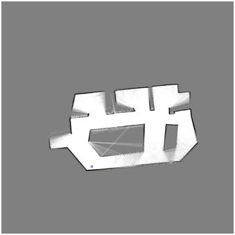
Fig. 19 Map generated at the later steps of the algorithm. It should be noted that the Fast SLAM algorithm corrects the map. The correction could be seen by comparing this map with the map in Figure 18.
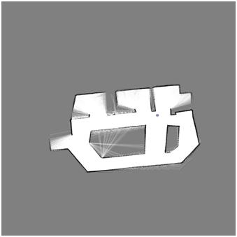
Fig. 20 Nearly completed grid map
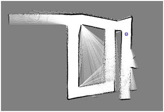
Fig. 21 Half complete Grid Map of our second map which is generated by our algorithm.
.
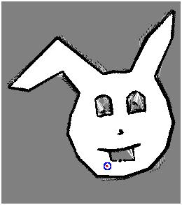
Fig. 22 Half complete Grid Map of our third map which is generated by our algorithm.
In all of our experiments we have observed that, the time complexity of the Fast SLAM algorithm is the main problem for real time applications. Although the time interval for the SLAM is 0.5 seconds for each motion performed, our simulator was in front of our algorithm.
We have also noticed that decreasing the cruising speed of the robot increases the SLAM efficiency in the map as the difference between sensor readings is less that a faster action performed. However, benefiting from a slow motion and increasing the particle count in the motion model does not yield a faster computation. Although more particles existing in the algorithm would increase the correctness of the whole system, it also increases the time complexity.
We also included the resulting map created by our Fast SLAM algorithm when only the raw encoder data from the Mobile Sim. Robot is used without any additional Gaussian noise.
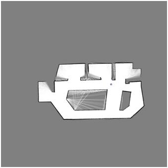
Fig. 23 Grid map created depending only on the raw encoder data of Mobile Sim robot
VIII. CONCLUSION
Fast SLAM with Occupancy Grid Mapping is a powerful technique when we do not have predefined landmarks. Resulting map is a complete map and have more information when compared to Fast SLAM using 2D EKF landmarks.
The main drawback of our algorithm is resources required. Since we have to store a 2D grid for every particle and since for an update sequence we need to update quite large portion of the grid it takes too much time and consumes too much space. With a naive implementation it becomes infeasible to use and it will not even be near real time.
Time requirements of this algorithm, limits the number of particle we can use, causing algorithm to lose its robustness. Some clever resampling techniques must be implemented to use in robotics given the technology we have today.
REFERENCES
[1] Thrun, Sebastian, Wolfram Burgard, and Dieter Fox. Probabilistic Robotics. Massachusetts Institude of Technology Cambridge, MA, USA: The MIT Press, 2005.
[2] Montemerlo, M., Thrun, S., Koller, D. and Wegbreit, B. "FastSLAM: A Factored Solution to the Simultaneous Localization and Mapping Problem." AAAI, 2002.
[3] Xianzhong, Chen. “An Adaptive UKF-Based Particle Filter for Mobile Robot SLAM”. International Joint Conference on Artificial Intelligence, 2009
[4] Montemerlo, M., Thrun, S. Simultaneous Localization and Mapping with Unknown Data Association using FastSLAM. ICRA, 2003
[5] MobileSim. http://robots.mobilerobots.com/wiki/MobileSim
[6] OpenCV. http://opencv.willowgarage.com/wiki/