Author: Utku Çulha
This web page consists of information about the tangent bug algorithm and its implementation. The content of the web page is indexed as below:
| Index | Subject |
|---|---|
| 1 | Introduction |
| 2 | Algorithm |
| 3 | Platform |
| 4 | Experiments |
| 5 | Observations |
Some of the images used in sections 1 and 2 are adapted from Asst. Prof. Uluç Saranlı's Robot Motion and Planning course slides and from chapter 2 of the book "Principles of Robot Motion" by Choset H. et.al.
The tangent bug algorithm is actually the imroved version of Bug1 and Bug2 algorithms. Unlike these methods, tangent bug algorithm depends on the existence of a range sensor that is mounted on the point robot in the map. By only investigating the output ot this range sensor, and including the knowledge of the robot's current pose and goal's pose, the robot plans actions to reach to the goal.
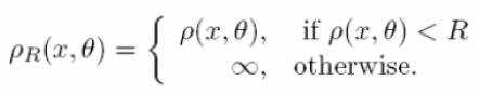
The range sensor mounted on the robot is a device that gives raw distance information from the robot to the environment covering the 360° circumference of the robot. The method in calculating the distance depends on the 'laser rays' that are emaneted from the robot's center to all degrees. One of the most important property of this raw distance sensor is that, only the distance to the closest obstacle on a particular laser ray is computed. The sensor could be modelled as follows:
where pR(x,ø) is the distance to the closest obstacle on a particular laser ray emanating from robot center at a degree of ø. It is also noticable that the sensor has a finite range 'R', and if there are no obstacles on a particular laser ray, the pR(x,ø) is returned to be infinity for that angle.
However, using such a dicretizing range sensor causes problems with respect to increasing distance. The length of the arc between two adjacent laser rays increase while R increases. This causes the loss of information about the obstacles that might intersect these arcs.
The more formal way of expressing the sensor model is:
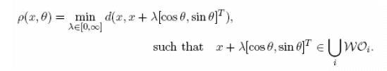
where x denotes the position of the robot and the set WOi denotes the obstacles that are found in the world of the robot.
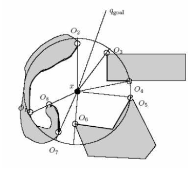
Depending on the range sensor data, the robot in the tangent bug algorithm is assumed to detect intervals of continuity. These intervals can be called as the continious set of points with having a discontinuity point at each end. These intervals can be both found in the free space ( sensed space without any obstacles ) and on the obstacles. The discontinuity points are the locations where the sensor information suggest that a continuity interval has ended and another interval has started. Figure 1.1 shows the discontinuity points in an enviroment, where Figure 1.2 shows the sensor data that depicts these points.
 |
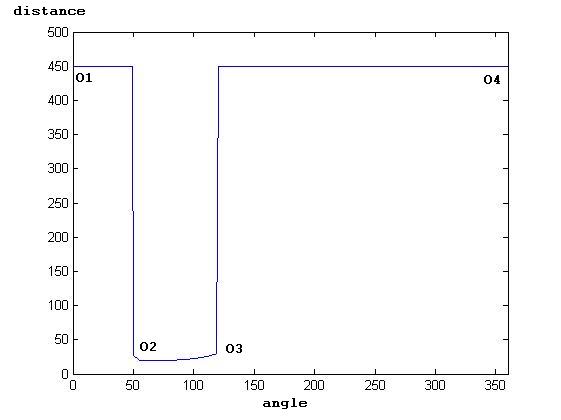 |
| Figure 1.1 The robot is denoted with x and the goal is qgoal. The discontinuity points are denoted as Oi | Figure 1.2. The data of the raw distance sensor suggests that there exists a continuity interval between degrees 0-50, 50-120 and 120-360. The sharp change in the distance between angles 50 and 120 shows the existance of an obstacle |
The tangent bug planner uses the data avaliable presented on the previous section. Depending only on these data, the planner finds a short way to the goal or announces failure if the goal is unreachable. On the overall the tangent bug planner consists of two switching planner states: motion to goal and boundary following.At the beginning of the planner the state starts with the motion to goal planner and switches to boundary following when necessary parameters hold.
This behaviour is activated either when there is no obstacle sensed on the direction from robot to the goal or the robot can find a decreasable heuristic distance from a followed obstacle to the goal.This sub-planner consists of 2 motion behaviours that are adapted by the robot. The first one is the trivial motion where the robot detects the direction to the goal and moves directly towards it while concluding that there exists no obstacles intersecting the line from robot to the goal. This motion keeps executed while sensor readings yield maximum range distance result for the angle corresponding to the direction to the goal.
The end of this trivial direct motion comes when the robot senses an obstacle on the direction to the goal. After this point, the sub-planner switches to the second part of the motion to goal behaviour. In this behaviour the robot detects points of discontinuity on the sensed obstacle. It is important to note here is that any discontinuity point that seperates a continuity interval of an obstacle which is located away from the direction to the goal is not a point of interest. Considering a scenario shown in Figure 2.1.
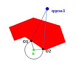
Figure 2.1. The robot is denoted with x, goal with qgoal and discontinuity points with O1 and O2. The lines connecting the robot to O1 to qgoal is dist1 and O2 to qgoal is dist2
the robot starts to calculate a heuristic distance to the goal computed as heur = d(x,Oi) + d(Oi,qgoal). At each step of this behaviour the robot finds points that will decrease this heuristic distance. When the robot finds that point, the robot starts to move towards that point, therefore in the belief of decreasing the heuristic distance. However at some stage, this heuristic distance cannot be decreased any more. This point is the triggering event for the motion to goal planner to switch to the boundary following planner.
In this part of the planner, the robot starts to compute two different distance parameters; dreach and dfollowed. In general dfollowed is the shortest distance between the point on the followed boundary ( among all of the sensed points since the beginning of the boundary following for this particular obstacle) of the obstacle and the goal. And dreach is the shortest distance between the points on the range of the robot ( this range includes both the points that are located on the followed obstacle and the points on the range of the sensor in the free space)
When the boundary following planner is initiated, the robot starts to move to the direction of the last Oi selected from the motion to goal behaviour. With the direction selected, the robot moves on the tangent line. This tangent line is perpendicular to the line that connects the robot and the point closest to the robot on the followed obstacle.
This sub-planner continues to execute while the following statement holds
dfollowed > = dreach
Whenever dreach falls below dfollowed, the robot switches back to the motion to goal behaviour
In order to implement the tangent bug algorithm I have used MATLAB ( simulation ) and CamStudio (video capturing). The world I have chosen is a continious world bounded with a closed box of 300x300 units. The robot and the goal are denoted as points on this space as robot = [Rx,Ry] and goal = [Gx,Gy]. The movement factor is 2 for the robot. The obstacles are denoted as polygons with differing sides and properties ( convex and non-convex). The sensor model has a maximum range of 30 units and yields an infinite response for free spaces with a value of 450 ( that value is selected as is longer than the diagonal of the bounding box ). I have selected the threshold for detecting obstacles as a change in the distance of 20 units between two angles.
The source code for the implementation could be found here.
I have implemented 5 different cases which the first 4 is a success case where planner finds the goal and the last one is a fail case.
In this case, both robot and the goal is located on the same line. The planner initiates the motion to goal planner at first and switches to boundary following after the obstacle is sensed. It should be noticable that after the robot finishes the first boundary following sequence it never continues a long term boundary following again. The reason for that is the the heuristic distance keeps on decreasing and whenever boundary following, the dreach parameter falls quickly below the dfollowed as robot approaches the goal at every step.
The main reason for implementing such a case was to show that planner chooses a direction and follows it strictly even if symmetric Oi's points yield same heuristic distances.
This case is much similar to case 1 apart from the distorted symmetry.
In this scenario, the robot faces a non-convex obstacle. The reason for creating such an obstacle was to test the planner whether it follows the behaviour of boundary following. It is noticable here is that after some time when robot starts boundary following, the robot falls apart from the obstalce for a minute. In other words, the sensor yields max reading. After that, robot switches back to motion to goal behaviour and moves directly to the goal. When ever it faces the obstacle again, it starts the boundary-following procedure.
This scenario is similar to case 3 apart from an added new obstacle that comes after the first one. The reason for creating the second obstacle was to test the repeatability of the planner algorithm.
Differing from the rest of the cases, this case is a scenario in which the goal is within the obstacle regions. It is expected for the planner to detect this end and announce failure. However, in my implementation the planner crashes at some point while covering the second phase of the boundary following sub-routine. I strongly believe that this crash is due to the wrong calculations of expected following angle. It can be noticed that, after the robot handles the first turn, it starts to diverge from the obstacle.
Apperantly the most challenging concept in understanding the concept was to find a good explanation to dreach and dfollowing. In the book of Principles of Robot Motion by Choset. H. et. al. and in all of sources which took the book as reference, the distinction between these parameters where not clear.
One important observation here is the boundary following distance. It can be noticed from the videos that the robot follows the obstacle boundaries nearly at the limit of sensor range. This offset sometimes causes distractions from obstacle boundary ( like in case 3 ) and the termination of boundary following procedure. I think this is caused of the sensor range and the movement factor together. As the movement factor is small, the robot cannot get close to Oi's during motion to goal procedure. And the Oi's detected by the sensor move too fast on the obstacle so that the triggering event for the boundary following procedure is occurs too before the robot can come close to the obstacle.
It should be noted here that, my definition of dreach might cause the behaviour of large turns at the corner points of obstacles. It is also observable that the tangent line finding function might work wrong ( because of the strictly followed Oi direction ) which causes the failure of the last case.
Utku Çulha - Bilkent University
Computer Engineering Department