Author: Utku Çulha
This web page consists of information about the potential and navigation function algorithms, their implementation and comparison. The content of the web page is indexed as below:
| Index | Subject |
|---|---|
| 1 | Introduction |
| 2 | Potential Functions |
| 3 | Algorithm |
| 4 | Platform and Source |
| 5 | Experiments |
| 6 | Observations |
Some of the images used in sections 1 and 2 are adapted from Asst. Prof. Uluç Saranlı's Robot Motion and Planning course slides and from chapter 2 of the book "Principles of Robot Motion" by Choset H. et.al.
Having explored the bug algorithms, the main idea of this assignment is to expand the path planning algorithms for a robot in a more complex world. Again, assuming a point robot, this web page investigates the improvements in potential functions and compares the performance of different algorithms. Based on the idea of physical rules in potential fields, potential functions assume the existance of repulsive and attractive forces acting on a point robot in its world. Here, the general motivation for the functions will be the expectation of a complete path planning algorithm that moves the robot by the vectoral sums of the attractive force of the target and repulsive forces from obstacles in the area.
In potential functions, the aim remains same while operation and configuration differ from the bug algorithms. The aim is to find a complete path from the starting location of the robot to the target location at the same time avoiding obstacles. Comparing with bug algorithms, it is seen that the configuration space in those algorithms is limited to two dimensions. However the potential functions that will be mentioned here can be applied to a more general class of configuration spaces.
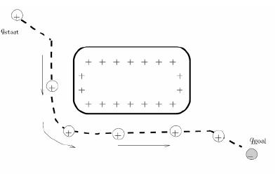
The potential functions that will be explored will be differentiable real values functions; so assuming the value of the potential function to be the energy, the gradient of this function will yield force. Depending on this simple but strong assumption, the gradient of the potential field will be expected to move the robot to the goal position. The success of the function depends on the attractive and repulsive potential gradients acting on the robot. The robot and the rest of all the obstacles are assumed to be positively charged, where the goal is negatively charged. This charge difference yields the repulsive forces pushing the robot and goal pulling it.
Figure 2.1 - Potential field and gradient forces acting on the robot to achieve complete path
It is important to mention here is that, the although potential functions could be used in higher order dynamics, the algorithms and implementations depend on first order systems so that potential gradient is velocity instead of force. Considering this choice, we can also extend our methodology by stating that the robot will follow a path downhill starting from a high ground to the goal which is located at the lowest ground in the world. This downhill action depends on the gradient descent algorithm, where robot follows the negated potential gradient.
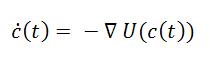
Equation 2.1 - Gradient descent shown as the negated gradient. U stands for the potential function
The potential function is the sum of attractive and repulsive potential functions on the robot. Gradient of this sum yields the total velocity of the robot at its current position.
![]()
Equation 2.2 - Total potential is summed of attractive and repulsive potentials
In this experiment two kinds of potential functions is implemented: additive attractive/repulsive potential and navigation potential functions. Each of these functions have differing gradients which result in different paths for the robot. It will be noticed that former of these potential functions will fail in getting stuck in a local minimum location where the latter potential will overcome this problem.
This potential function consists of the summation of attractive and repulsive potentials on the robot.
There are several important functions and definitions needed to be defined before explaining the details of the following equations. Attractive potential, Uatt, is required to be monotically increasing, therefore there are several choices to implement. The first one is the conic potential where distance from the robot to the goal is calculated in means of Euclidian distance scaled with a constant parameter. The other choice is the quadratic potential defined to overcome the discontinuties in the gradient vectors caused by world configuration. With respect to the overshoot of the robot near the goal, the algorithm will make a decision between the implementation of these potentials. Given a predefined distance threshold dgoal*, conic potential will be used when d (q,qgoal) , i.e, the distance between the goal and robot, is larger than dgoal* and quadratic potential will be used otherwise.
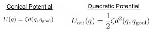
Equation 3.1.1 - Conical and quadratic potentials that will be selected with respect to the distance from the robot to the goal
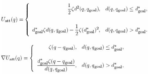
Equation 3.1.2 - Combined attractive potential function and gradient function with the distance relation
In the equations above, ζ is the scaling factor and dgoal* is the threshold value that defines the distance between the robot and the goal which will be compared for the choice between conic and quadratic potential. It is important to to here that gradient of the distance function ζd(q,qgoal) is defined as ζ (q - qgoal ) / d (q,qgoal)
As there is exactly one goal in the world, attractive potential is calculated upon the relation between the robot and goal only. However, including the bounding sphere in the world, there are numerous obstacles which affects the robot. So in order to calculate the total repulsive potential, the algorithm looks at the relation between the robot and every obstacle. Same as the attractive potential, there are predefined parameters in repulsive potential too. Considering many obstacles, the algorithm prefers to neglect the repulsive force of the obstacles that are too far from the robot. In order to define this distance, a proximity threshold Q* is used in the following algorithms. Also a scaling factor ŋ is used to define the scale of the potential velocity.
An important point in implementing the repulsive potential is to take care of repulsive forces of obstacles that are equally at the same distance to the robot. As this might oscillatory motion in implementation, the distance to the individual obstacles are preferred rather than the distance to closest obstacles. The following functions explain the repulsive potential and its gradient.
![]() ,
, ![]()
Equation 3.1.3 - Distance from the robot to the closest point in each individual obstacle and gradient of this distance
Equation 3.1.4 - Repulsive potential function. Notice that function neglects effects of obstacles located far from the robot
Equation 3.1.5 - Repulsive gradient function

Equation 3.1.6 - Total repulsive potential field
Another kind of a potential function is a navigation function. With respect to the failure of the previous potential function,whose results will be shown in section 5, this function is introduced. Unlike the previous one, there exists only one minimum point in the configuration space, so that there is not any local mimimum problem. Similar to the previous potential function, the gradients here are defined upon distance functions. In the sphere wolrd that the robot and obstacles stay, here are the distance functions.
![]()
Equation 3.2.1 - ßi shows the distance to obstalces. Note here that i = 0 is the bounding sphere
In the same fashion of adding attractive and repulsive forces, we obtain the total force acting on the robot. Following formulas are the attractive and repulsive gradients. Reader should notice here is that there is only one predefined parameter here. K is used in the repulsive gradients to ensure that there is exactly one minimum point that is the goal point. Increasing K will yield success of navigation function where decreasing the parameter will converge to the performance of the previous potential function.
 |
Equation 3.2.2 - Attractive and repulsive potentials respectively
Combining both of these attractive and repulsive potentials we have the following total potential. The graident of the total potential yields the forces acting on the robot in the sphere world.
![]()
Equation 3.2.3 - Navigation function in the sphere world
Equation 3.2.3 - Gradient of the navigation function
|
|
|
|

Equation 3.2.4 - Resulting gradient of navigation function
I have used MATLAB to implement the potential functions. For both of the potential functions sphere world is the same. The world is defined as world = [ x0 y0 r0 , x1 y1 r1 ...], where the first row is the bounding sphere and the rest is the obstacles. For the sake of simplicity and convergence time I have defined the bounding sphere to have a radius of 15 with origin located at [0,0]. The position of the goal and robot is changed for each experiment ( 1. simple, 2. composed, 3. local minimum ) but each of these configurations remained same for both of the potential functions. I have chosen the required parameters for both functions by trial and error. For the first potential function, the parameters are as follows: ζ = 0.5; dgoal* = 15; ŋ = 1; Q* = 1. For the latter function K = 3.
I have used MATLAB's ode45() differential equation solver. In order to control the integration and terminate it, I have also implemented event functions for ode45. These event functions actually implemented in order to detect whether robot has reached the goal or is stuck in local minimum point. These detections required a threshold parameter, Є, which is 10e-01 for former function, 10e-05 for the latter function.
The source code for the whole implementation could be found here.
I have implemented 3 different types of world configurations in order to compare the performace of 2 potential functions. Those configurations started from a simple case, then a more composed one and at the end the local minimum configuration. For each of the experiment results below, the configuration space will be shown at first. Then the resulting path from additive potential function and potential field that yielded that result will be shown. After that the convergence time will be expressed. After that, results for the navigation function will be expressed in the same order.
In this configuration there are only 2 obstacles found in the sphere world which occlude the direct path to the goal. The world is defined as world = [0 0 15; 1 1 2; -5 -7 3 ]. The locations of robot and the goal is [-3 -11] and [-1 5] respectively.
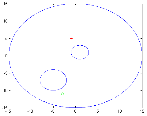
Figure 5.1.1 - Configuration space for the first experiment. Blue circles represent the obstalces. Green circle is the robot and red star is the goal.
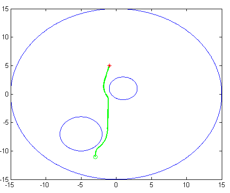
Figure 5.1.2 - Resulting potential function path
 |
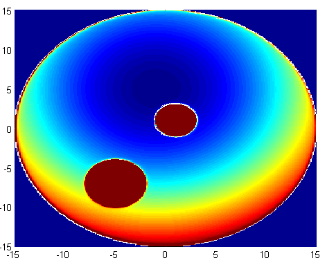 |
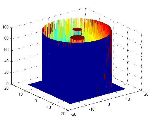
Figure 5.1.3 - Potential field that generates the resulting path. Notice that goal is located at the minimum point here which is shown with cold blue areas. Red areas represent higher grounds in the sphere world
The convergence time for the robot to reach the goal is 0.078143 seconds.
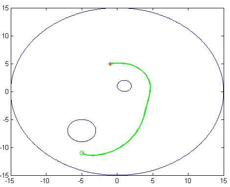
Figure 5.1.4 - Navigation function yields the path above
 |
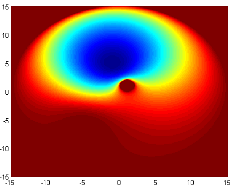 |
Figure 5.1.5 -Potential field in navigation function. Notice that an increased K lets the goal to be at the bottom of the bag which can be seen better in the figure on the left
The convergence time for the robot to reach the goal is 0.069226 seconds.
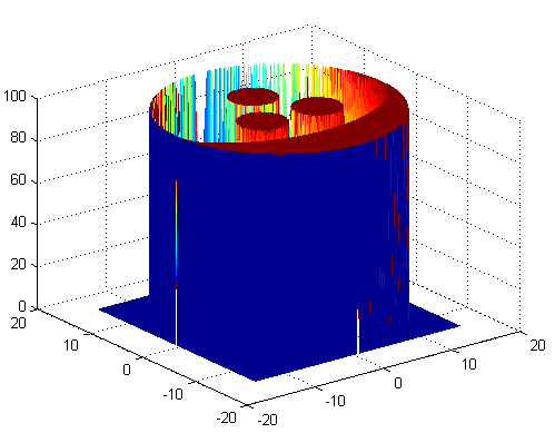
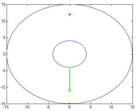
In this configuration there are 3 obstacles found in the sphere world which occlude the direct path to the goal. The world is defined as world = world = [0 0 15; -3 -6 2; 2 1 3; -3 7 2]. The locations of robot and the goal is [-3 -11] and [-1 12] respectively.
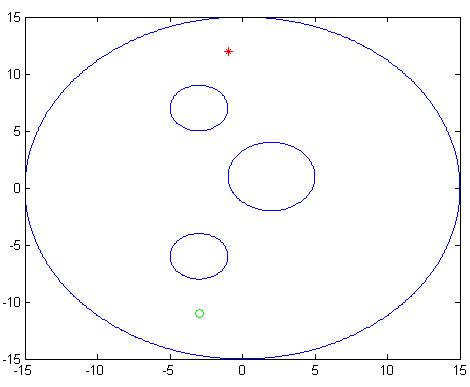
Figure 5.2.1 - Configuration space for the second experiment. Blue circles represent the obstalces. Green circle is the robot and red star is the goal.
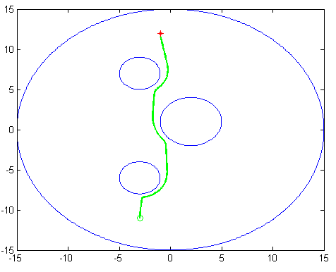
Figure 5.2.2 - Resulting potential function path
 |
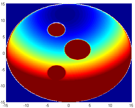 |
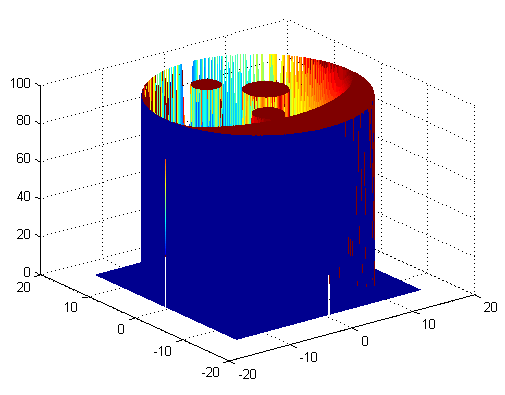
Figure 5.2.3 - Potential field that generates the resulting path. Notice that as the position of the goal changes, the attractive potential field changes. Compared to the first experiment, we now have a more sloping downhill towards the goal
The convergence time for the potential function is 0.167987 seconds.
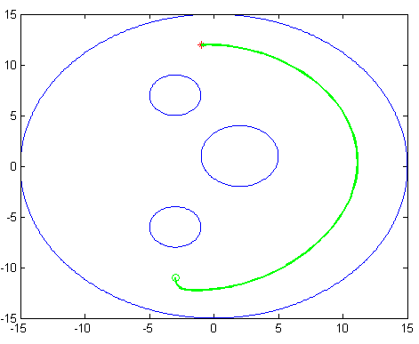
Figure 5.2.4 - The resulting path of the navigation function
 |
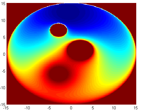 |
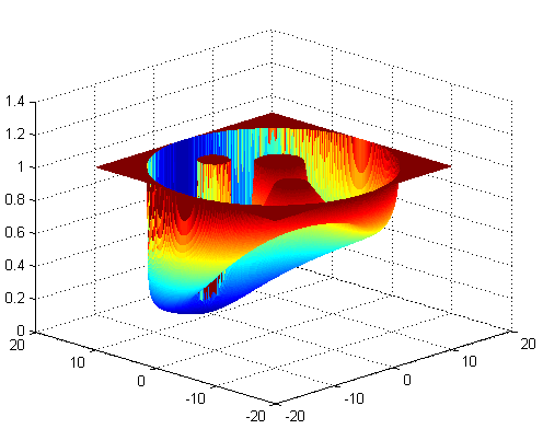
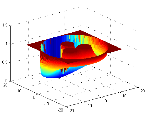
Figure 5.2.5 - Navigation function field yields one local minimum which is the goal point
The convergence time for the robot to reach the goal is 0.114136 seconds.
In this configuration there are 3 obstacles found in the sphere world which occlude the direct path to the goal.What is more the aim here is to create a local minimum area that will lead former potential function to fail and get stuck at this local minimum point. The world is defined as world = world = [0 0 15; -4 -2 3; 4 -2 3; 0 5 3]. The locations of robot and the goal is [-1 -11] and [0 12] respectively.
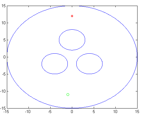
Figure 5.3.1 - Sphere world with local minimums between obstacles
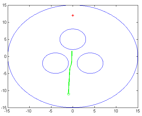
Figure 5.3.2 - Former potential function fails as expected at one of the local minimum points. ode45() stops integrating as local minimum event has been detected
 |
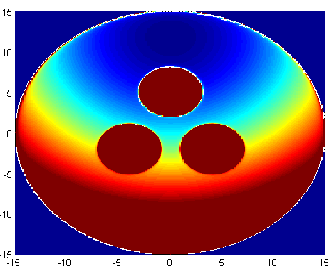 |
Figure 5.3.3 - Notice the local minimum points between the obstacles in the figure on the right. Although the global minimum is still the goal, function fails to get the robot to the goal
The function fails to reach the goal so we cannot mention the convergence time. However the function stops integrating after 0.047061 seconds when the local minimum problem has been detected.
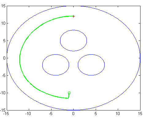
Figure 5.3.4 - Navigation function succeeds in finding the path to the goal despite the local minimum areas
 |
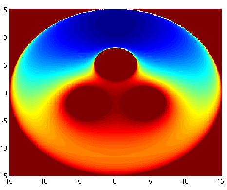 |
Figure 5.3.5 - Navigation function fields show local minimum areas
The convergence time for robot to reach the goal is 0.001401 seconds.
When we compare both of the functions we can see that navigation function outbeats the additive potential function both in convergence time and success rate. A comparison table showing the convergence times can be seen below.
| Additive Potential Function | Navigation Potential Function | |
|---|---|---|
| Simple Case | 0.078143 sec. |
0.069226 sec. |
| Composed Case | 0.167987 sec. |
0.114136 sec. |
| Local Minimum Case | Inf. |
0.198178 sec. |
Table 6.1 - Performance comparison of two functions
Although its low performance, additive potential function is easier to implement with respect to its comparible easy gradient and potential formulas. However, MATLAB helps the user to implement both of these functions with its heavy support on integration functions.
Using ode45() in order to perform integrals for the acting forces, increases the efficiency of the functions considerably. It is most likely to observe longer convergence times for functions when manual in-loop integration is performed. What is more ode45() function enables to integrate event functions in order to detect possible termination points. Reaching the goal, getting stuck at the local minimum has been implemented by using event functions of the ode45() function.
In this part another comparison between two functions has been made with a given interesting configuration. Building the world with only one obstacle which is located on the direct line from the robot to the goal also leads the failure of the additive potential function. Here are the results.
 |
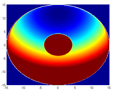 |
Figure 6.1 - Additive potential function fails to find the path
Navigation function also fails to find the path in this case and fails to detect the terminating event because of the choice of Є. The possible reason for this result is the vectoral summation of forces acting on the robot. As the world is sphere shaped, forces acting on opposite directions but existing on the same line cancel each other out. Because of this reason the robot stays at the same position. Any smallest change at the position of the robot or the goal would yield a successful path. The proof of this theory is shown with a change of 0.2 units for the robot's initial pose applied in the additive potential function.
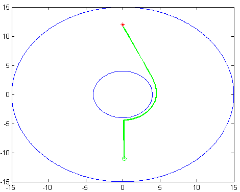
Figure 6.2 - Resulting potential function path with a given 0.2 displacement of robot for its initial location
Utku Çulha - Bilkent University
Computer Engineering Department