
Author: Utku Çulha
This web page consists of information about the visibility graphs and their implementation. The content of the web page is indexed as below:
| Index | Subject |
|---|---|
| 1 | Introduction |
| 2 | Visibility Graph Approach |
| 3 | Algorithm |
| 4 | Platform and Source |
| 5 | Experiments |
| 6 | References |
Some of the images used in sections 1 and 2 are adapted from Asst. Prof. Uluç Saranlı's Robot Motion and Planning course slides and from the book "Principles of Robot Motion" by Choset H. et.al.
Building up on the previous approaches in robot motion planning, this implementation investigates the details of visibility graph algorithm. So similar to bug algorithms, the world that our robot lives in is a 2D environment with polygon based obstacles. These obstacles can both be convex and concave where the most important difference from other approaches is that the robot is now a triangular shape instead of a point. Considering this robot volume, visibility graph approach focuses on an important space transformation where workspace obstacles are expanded into configuration space obstacles. As its name suggests visibilty graph approach forms a configuration space and finds visible node connections in this space. After finding the connections between obstacle vertices, the approach lets the robot to traverse a graph based search algorithm such as A* search.
As defined briefly above, visibility graph approach is applied in a 2D world with polygon shaped obstacles which aims to find the shortest path between the start and goal points by moving a polygon shaped robot. The main difference of this aprroach from the previous ones is the robot's shape. As the robot was considered to be a point in Bug algorithms, the workspace obstalces were the same as configuration space obstacles. However, in our case configuration space obstacles are expanded from workspace obstacles because of the polygon shape of the robot. Another important notice here is the shape of the obstacles. Normally visibility graph approach lets convex polygons as obstacles. However by the help of triangulation methods, concave obstacles could also be used. Delaunay Triangulation, which will be explained in the algorithm section, will take concave polygons and convert them into many small triangles which are all convex polygons by themselves. The general method of converting workspace obstacles into configuration space obstacles in performed by the Star Algorithm which will also be explained in the next section.
The idea of forming a configuration space is leading the aprroach to create a graph by using the nodes, i.e. vertice and edges of configuration space obstacles, in the 2D world. Having formed a configuration space, the shape of the robot is then being included in the obstacles. This lets the algorithm to accept the robot as a point from then on. In this point of the algorithm, all we have is vertices of obstacles, the start and goal points and edges of obstacles. Having only these elements, a graph can easily be constructed by connecting the mutually visible elements. The name of the approach comes from this contruction, where visible nodes are connected to create graph lines.
After creating a graph, any graph based search algorithm becomes suitable for the aim of the approach. But before starting any search algorithm, the graph is required to be revisited. The result of visibility graph includes many unnecessary edges that will increase the search time while performing a graph based search algorithm. Therefore, reducing the graph nodes becomes an important operation in order to increase efficiency of the whole approach. The book suggests an algorithm called Rotational Plane Sweep Algorithm and the idea of Seperating and Supporting Lines in order to cope with the reduced visibility graph problem. For more information about these approaches the reader may consider revising the relevant chapters from the reference book [1]. However, I have applied a custom technique in order to accomplish a reduced visibility graph, which will be explained in the next section.
The last step in the whole visibility graph approach is to apply a graph based search algorith. Because of its completeness and efficiency A* Searh Algorithm is preferred for this role. Given a graph as input, this algorithm produces a back track from the goal towards the starting point following each nodes visited. This path is generally unique and accomplishes the shortest path possible concerning the whole node probabilities. The details about the A* search algorithm is given in the next section.
|
|
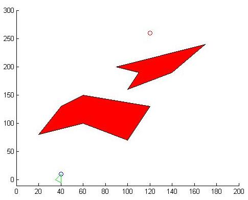
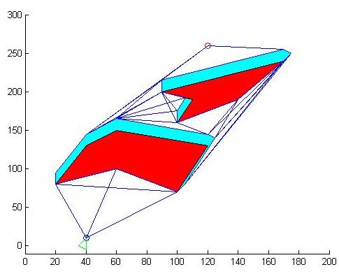
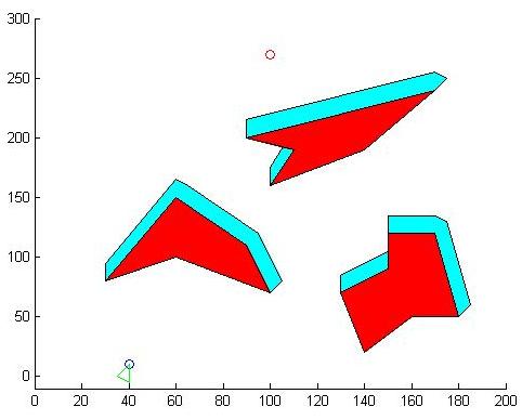
Figure 2.1 - Figure on the left shows an example 2D world configuration with 2 concave obstacles shown in red polygons. The robot is shown with a green triangle whose vertex is located on the starting point shown with blue circle. The goal point is shown with a red circle. The figure on the right shows the resulting configuration spape formed concerning the workspace obstacles and the robot. This result of star algorithm is shown with cyan expansions to the workspace obstacles.
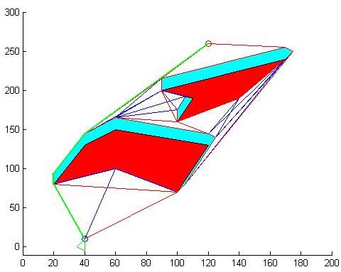
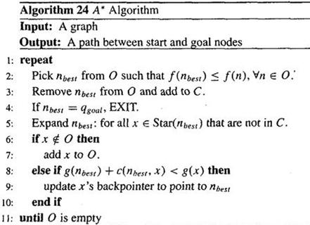
Figure 2.2 - The resulting graph nodes and shortest path. The blue lines represent the result of visibility graph, where red lines show the reduced graph. The thick green line is the result of A* algorithm and shows the shortest path.
In this part, the algorithms that build up the visibility graph approach will be explained in required detail. I will explain the algorithms I have implemeted and used in the sequential order they are used in the whole approach.
The star algorithm is based on finding the intersection points of two polygons in a 2D world. For our case these two polygons are stable convex or concave obstacles and a portable robot polygon. In order to understand the cases in polygon intersection, the representation below must be understood.
 |
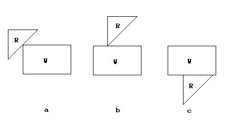 |
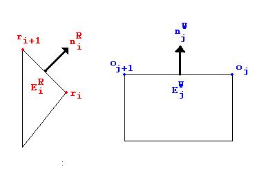
Figure 3.1 - The figure on the left shows the edge, normal and vertex representations both for the triangular robot and rectangular obstacle. The figure on the right shows 3 kinds of intersection cases between the robot and obstacle.
One important notice here is that robot is only allowed to translate, in other words the configuration space is built with a predefined robot angular position. Considering this rule and the 3 types of intersections above, the star algorithm conducts the following applicability rules.
![]()
![]()
Rule 3.1 - Applicability rule applied when an edge of the robot and a vertex of obstacle intersects
![]()
![]()
Rule 3.2 - Applicability rule applied when an edge of the obstacle and a vertex of the robot intersects
For the third case where an edge of the robot and an edge of the obstacle intersects, both of these rules apply at the same time. The main idea of the star algorithm can be better explained visually.
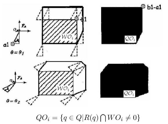 |
|
Figure 3.2 - The figure on the left shows the expansion of workspace obstacles into configuration space obstacles with given 2 different robot poses. An important point here is the location of the coordinate frames attached to the robot. The figure on the right is the result of star algorithm in my experiments. The coordinate frame here is located on the vertex of the robot which is located on the starting point.
However, there is one draw back of the star algorithm; it works on convex polygons. In order to improve the visibility graph approach, concave obstacles should be included. In order to accomplish this, another important process is required. This process is called Delaunay Triangulation which aims to create smaller tirangles out of convex and concave polygons.
Basically delaunay triangulation is a process where for a given polygon the minimum number of triangles that make up this obstacles are found. The idea is very applicable to our problem because by this method concave obstacles can be turned into triangles, which are all convex shapes, and star algorithm can be applied. This very useful method used in computational geometry can be found as a built-in function in MATLAB as delaunay(). Details about the algorithm[2] and MATLAB implementation[3] could be found on the web.
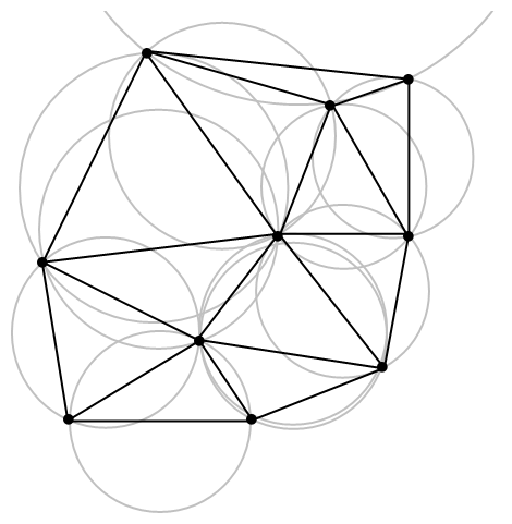 |
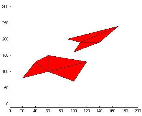 |
Figure 3.3 - The figure on the left adapted from Wikipedia[2], shows the idea behind triangulation in a polygon. The aim here is to find the minimum number of triangles with each having possibly large angles. The figure on the right is the triangulation results in my experiments. The MATLAB function delaunay() produces such triangles out of concave obstacles.
Delaunay triangulation is used as a part of star algorithm in my experiments. The triangles found in this method is then given to star algorithm as unique convex obstacles. Then these obstacles are transformed into configuration space obstacles. Any configuration space obstacle which has a connection with another obstacle is converted into a single obstacle.
Construction of visibility graph and its reduced version is explained with rotational sweep line algorithm in the reference book[1]. The main idea of this algorithm is creating a virtual horizontal axis for each vertex in the configuration space, including the start and goal points, and create lines emanating from this vertex connecting to the other vertices in the space. After that sorting these lines, eliminating the lines which have intersections with other obstacles yield the visibility graph. What I have used in my experiments is a similar algorithm except that the horizontal axis and sorting. For each vertex in the configuration space, unique lines that connects this vertex to other vertices are found. After that, any line which have an intersection point more that 2 is deleted from the graph.
For a given visibility graph, supporting and seperating lines are used for reduction in the reference book. The main idea of these lines is to find tangent lines between and around the obstacles. Any lines that fall apart from these lines are eliminated. These lines actually represent the shortest path from one obstacle vertex to the other obstacle. In my algorithm, I have increased the lengths of the connecting lines found in the visibility graph. If an increased line still has 2 intersection points, these lines are suitable for reduced visibility graph. Other lines which fail to have only 2 intersection points are observed to be non-tangent lines between vertices.
 |
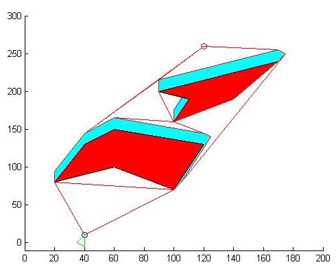 |
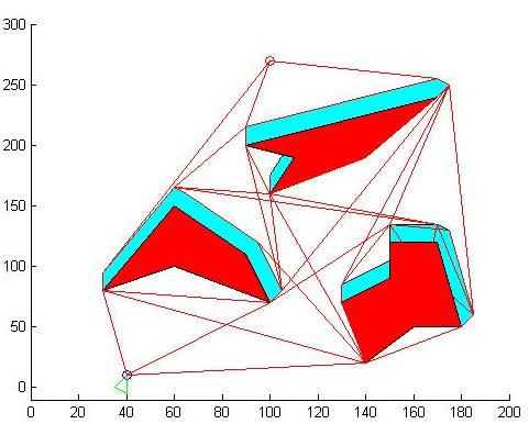
Figure 3.4 - The figure on the left shows the resulting visibility graph. The figure on the right shows the reduced graph. Notice that some of the obstacle edges are eliminated during this process.
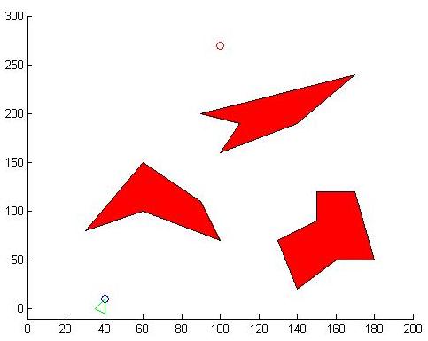
A* search is a best first graph based search algorithm that finds the shortest path between two nodes in the graph. An important function used in this search algorithm is a heuristic information that leads the search towards the goal. This heuristic information is an estimate about the distance to the goal in our case. Where many data could be used as heuristics, in visibility graph approach the Euclidian distance between the current node and the goal is preferred.
The search algorithm starts with an initial number of nodes that are neighboor to the starting point. In each iteration algorithm looks for the value of a function f(n) = g(n) + h(n) for each node n. This value is the sum heuristic about the distance to the goal and the real distance covered so far in order to reach that node. For each node with a value of function f(n), the algorithm selects the node with this minimum value and expands the neighboors of this selected node n. During the process, any node which has the minimum value of f(n) is selected.
A* search also remembers the nodes visited in each iteration. This memory both avoids the re-visiting of nodes and is used for back tracking when the shortest path is found between the start and goal nodes. With the notations given, the A* search algorithm is as below.
O = Open set, or priority queue which includes the nodes that are subject to search at an iteration step
C = Closed set, the visited nodes so far
c(n1,n2) = the length of the edge connecting n1 and n2
g(n) = total length covered so far in order to reach node n
h(n) = heuristic cost function, or the Euclidian distance from node n to goal
f(n) = g(n) + h(n) main criteria for search and selection evaluation
 |
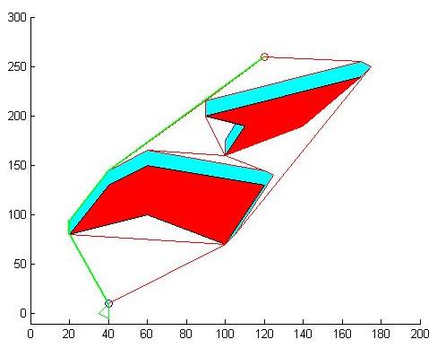 |
Figure 3.5 - A* search algorithm adapted from the reference book. The figure on the right is the shortest path found in my experiments. The thick green line shows the result of the a* search.
I have used MATLAB in order to implement the visibility graph approach. delaunay() function has been used to perform the delaunay triangulation process. Polygon intersection, union and coverage checks have been performed by the strong support of MATLAB's built-in functions. The source code for the implementation could be found here.
 |
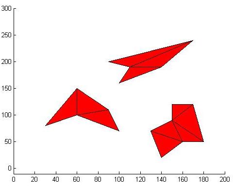 |
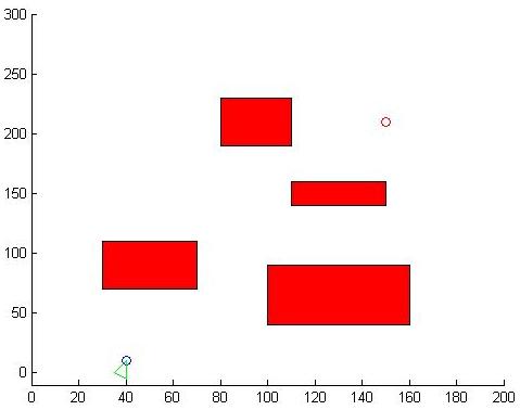
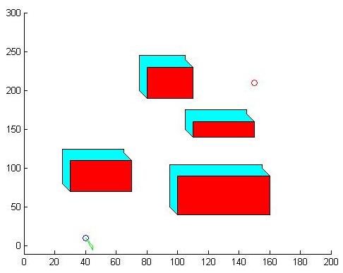
Figure 5.1 - Experiment 1 workspace and delaunay triangulation results
 |
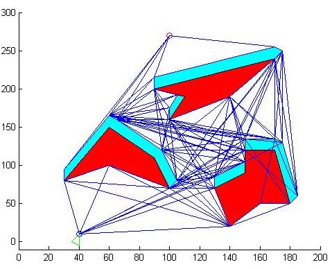 |
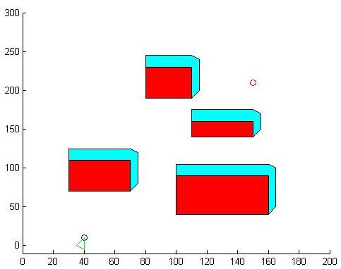
Figure 5.2 - Experiment 1 configuration space obstacles and visibility graph results. Notice there is a small error in lines in the righmost bottom obstacle
 |
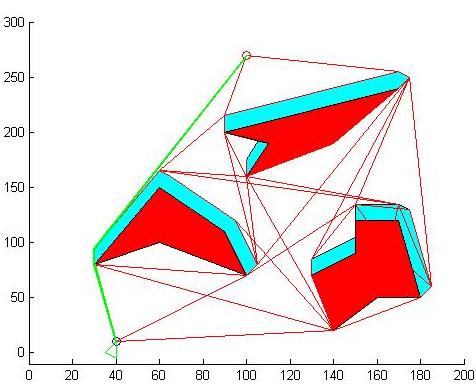 |
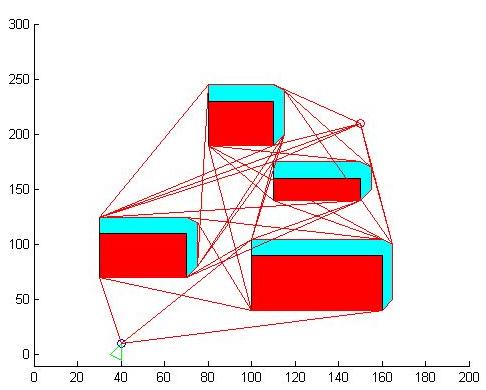
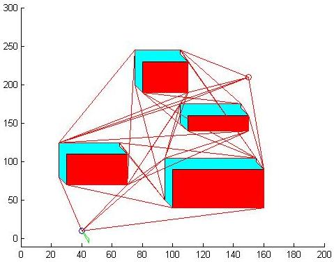
Figure 5.3 - The reduced visibility graph and the green line on the right shows the shortest path found.
 |
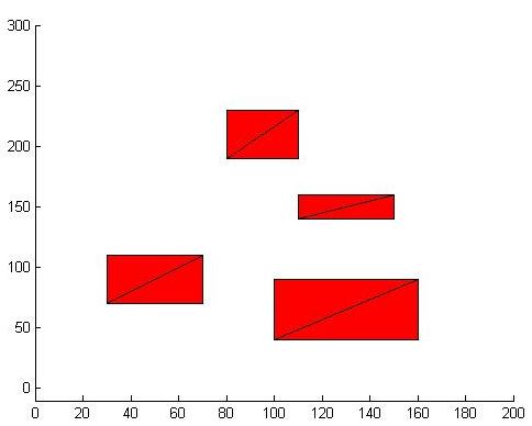 |
Figure 5.4 - Experiment 2 workspace obstacles and resulting triangulation
 |
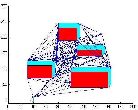 |
Figure 5.5 - Experiment 2 configuration space obstacles and visibility graph. The same error occurs here
 |
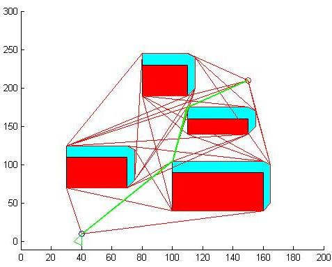 |
Figure 5.6 - Reduced visibility graph and shortest path found
 |
 |
Figure 5.7 - Experiment 3 with a different sized robot
 |
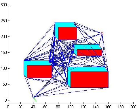 |
Figure 5.8 - Resulting configuration space obstacles and visibility graph, the error is still occuring
 |
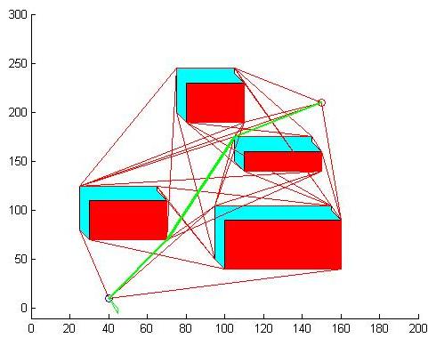 |
Figure 5.9 - Reduced visibility graph and shortest path
In all of these experiments, the error occuring in the top most edge of the obstacles are the result of a case of intersection that is forgotten to be implemented. Despite this small error, the visibility graph approach as a whole works successfully and eventually a shortest path is found. A nice song that represents these kinds of errors could be found here.
[1] "Principles of Robot Motion" by Choset H. et.al. Ch:5 Pg: 111-117
[2] "Delaunay Triangulation". Wikipedia, http://en.wikipedia.org/wiki/Delaunay_triangulation#cite_note-Delaunay1934-0
[3] "delaunay()". The MathWorks, http://www.mathworks.com/access/helpdesk/help/techdoc/ref/delaunay.html
Utku Çulha - Bilkent University
Computer Engineering Department