Author: Utku Çulha
This web page consists of information about the probabilistic roadmaps and their implementation. Among possible probabilistic methods, I have preferred to implement the PRM algorithm with some modifications on the sampling and roadmap construction part. The content of the web page is indexed as below:
| Index | Subject |
|---|---|
| 1 | Introduction |
| 2 | Probabilistic Roadmaps |
| 3 | PRM' Algorithm |
| 4 | Platform and Source |
| 5 | Experiments |
| 6 | Observations |
| 7 | References |
Some of the images used in sections 1 and 2 are adapted from Asst. Prof. Uluç Saranlı's Robot Motion and Planning course slides and from the book "Principles of Robot Motion" by Choset H. et.al.
Having explored various robot motion control methods, in this assignment probabilistic roadmaps will be investigated. This kind of aprroach has some differences from and similarities to the previous methods as well as brand new ideas implemented. The main idea in probabilistic roadmaps is to start with sampling the robot's many configurations in the known map. By this sampling process, the knowledge about the map differs from the tangent bug algorithms where looks similar to other methods. However the idea of sampling robot configurations is completely new and is special to this approach. The probabilistic term comes into role during this sampling process while a probabilistic function is used to generate robot configurations. The necessity for such an approach arises from the increased dimensions and calculation time for generating configuration free spaces for more complex robots and higher dimension worlds.
Without generating a configuration free space, probabilistic roadmap approach finds sample robot configurations where robot is collision free. After this generation, a roadmap between the found samples is created for the use of graph algorithms. This roadmap then becomes the unidirected graph for any graph based search algorithm, which consequently finds the shortest path from the start location to the goal location.
When the previous approaches, Tangent Bug Algorithm, Potential and Navigation Functions, Visibility Graphs, are investigated, it is noticed that each of these algorithms are sufficient only in restricted environments. The most striking of these restrictions is the dimension size of the world and the robot's shape. When the dimension of both of these increase, the methods mentioned above fail completely or converge to infinite time in calculation.What is more another problem defined in the latest algorithms, i.e. the necessity to find the configuration space from the workspace, becomes a hard challenge to cope with for robot configurations having multiple rigid bodies linked to each other.
When the assumption of the known world is taken as granted, probabilistic roadmap approach seems to solve these problems in a considerable time period with a probabilistic completeness. The assumption of knowing the workspace obstacles and their configurations lets the probabilistic roadmap methods to define a new sampling strategy to overcome the configuration space problem. This strategy depends on the probabilistic function chosen to generate multiple sample robot configurations in the known workspace. While finding possible collision free robot configurations, this strategy also succeeds a probabilistic completeness. Despite the space allocation and memory requirements to store the generated samples, this probabilistic completeness results in a successful motion planner for such an unrestricted world and robot configuration.
The sampling methods used in probabilistic roadmap approaches define different algorithms such as basic PRM or OBPRM. What comes after the sampling does also define different algorithms such as RRT. While RRT constructs a tree out of these sample nodes, PRM and similar methods create unidirected graphs. All of these algorithms aim to find a complete path from the start state to the goal state with minimum distance covered.
Among differing methods of basic roadmap planners, I have selected to implement basic PRM with some modifications in the sampling and connection phases in the overall algorithm. The next section explains the details of this custom PRM as well as the basic coordinate and world environment explanations.
The basic PRM algorithm is explained in detail in the reference book [1]. However if we want to summarize the method, it can be said that PRM method is built up of several sub-steps. In general PRM method starts with creating a number of robot configuration samples in the workspace. Having checked the collision free configurations, then PRM connects these samples, nodes from now on, to other nodes while still checking for collision free transitions. Each transition is called an edge and the number of these kind edges are found from the neighbooring k other nodes. Up to this point, all of these sub-steps are called as construction phase where collision free robot configuration and collision free edges are found by local planner and k nearest neighboors are found with respect to a distance function in the roadmap construction step.
The next phase in the overall algorithm is to find the, if existing, possible shortest path from the start state to the goal state. As the roadmap construction phase outputs a unidirected graph vith sample robot configurations as nodes and collision free paths between each node as edges, the query phase searches this graph for a suitable solution.
The subsections below shows my preferred approaches in each of the sub-steps mentioned above.
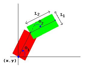
However the general approach can support multiple linked complex robots, with respect to the assignment I have used a robot with 2 rigid bodies linked to each other at a signle point. Therefore the configuration space of the robot is R^2*S^1*S^1 and any robot state is represented by q = [x y θ1 θ2]. θ1 is the clockwise angle from coordinate frame attached to the world at point (x,y) = (0,0) to the midline of robot's first rigid body. θ2 is the clockwise angle from the midline of robot's second rigid body to the first body's midline. These representations can clearly be seen in the following figure.
Figure 3.1.1 - Robot configuration. Notice θ2 is in the negative direction for this case
The red block shows robot's first body and green block shows the other where the thin black lines passing inside these blocks are the so called midlines. The parameters L1 and L2 are fixed values of the chosen robot and are 4 and 8 units respectively.
The big blue point where the coordinate frame is attached is the assumed robot base and the end points of each midline shows the reference points which will be used later in the convex hull construction. The robot's body parts can collide with each other, in other words -π ≤ θ1 ≤ π and -π ≤ θ2 ≤ π
Same as the robot configuration, despite the fact that the approach can handle high dimension worlds, in this assignment I have implemented a 2D world configuration consisting of multiple polygonal obstacles and a covering bounding box. The obstacles and the bounding box could easly be turned into circular shaped objects similar to the implementation in the potential function comparisons.
Having explained the robot and world configurations, the details about the PRM' can now be given. As said before the construction phase is the sub process which takes in the start and goal states of the robot and the workspace and outputs a roadmap which is a unidirected graph with sample robot configurations as nodes and the state transitions as edges. This process consists of two steps which are local planner step and roadmap construction step.
The local planner I have used in the PRM' approach is a more comprehensive planner than the planner mentioned in the reference book. This is one of the modifications I have done on the overall algorithm. The local planner starts with randomly sampling robot configurations in the free workspace. The random generation method I have used here is MATLAB's rand()[2] method which uses the Mersenne Twister algorithm by Nishimura and Matsumoto [3][4]. This method generates double precision values in the closed interval [2^(-53), 1-2^(-53)], with a period of (2^19937-1)/2.
I have made an important decision while using the random generator in the local planner. At first, each new sample was generated based upon the previous sample's configuration. In other words, the new configuration of the new sample depended upon the precision of the random generator with a given range parameter around the location of the previous sample. However, I have noticed that this kind of sampling approach decreases the probability of having samples in different locations in the workspace. A more detailed discussion about this subject has been done in the Observations heading. The current sampling algorithm in the working implementation is independent of previous samples. Therefore, the probability to have robot samples in different locations in the map is higher.
The sampler algorithm produces random locations for x and y parameters of the robot's base point. Also sampler produces random angles for θ1 and θ2 in the range of -π ≤ θ1 ≤ π and -π ≤ θ2 ≤ π. Considering these, checking only robot's x and y points for collision is not enough as the robot is a more complex polygon.
While generating samples, the local planner also checks for collisions between the candidate robot configuration and the map. I have used MATLAB's default polybool() function to check polygonal collisions[5].
The collision checker algorithm I have implemented, starts with checking possible collisions between 2 rigid bodies of the robot and the boundary box for each configuration sampler produces. This boundary checker also avoids samples created outside the boundary box. Because of the robot's polygonal shape, eventhough the base point of the robot stays inside the boundary, the configuration with respect to θ1 and θ2 parameters may have placed the rest of the robot outside the restricted map.
If the boundary check shows that there is no collision, the rigid bodies of the robot are checked for collision with workspace obstacles. The polybool() function is used here for obstacle and robot configuration collision.
Up to this point collision checker controls whether the new generated robot sample has a collision with any of the obstacles and the boundary box. What I have customized in the local planner is to add a convex hull checker to control whether the path covered during the state transition from the previous state, which has been accepted as a collision free state, and this newly generated state. This extra control ensures that there is exactly one collision free edge between generated samples. If though in this way, the PRM' algorithm's sampler looks familiar to the visibility-based sampling. In order to understand the effect of the convex hull checker, the idea of convex hull and its implementation in my approach will be explained.
Convex Hull Checker
The idea of convex hull is widely used in computer graphics in order to find the minimum polygonal shape covering a set of points in the given space. The details about the convex hull can be found in the web.[6] I have used this idea and modified it in my implementation to find the path covered during a state transition in the roadmap. As both the rigid bodies' position and orientation changes during the motion between one state to another, a complex polygonal shape is being formed. One of the suitable ways to check whether the robot does not collide with any obstacle during this change is to find the convex hull.
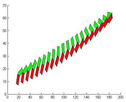
The convex hull checker generates a number of transition states between the real two states. The end points of the rigid bodies in all of these states are collected to form the convex hull polygon. The number of the transition states is a parameter that is possible to affect the success of the general algorithm. This parameter change is being discussed in detail in the Experiments heading.
 |
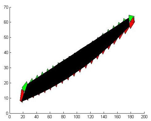 |
Figure 3.3.1 - The figure on the left shows the starting state, the transition states and the goal state. The transition states are generated by the convex hull checker. The figure on the right shows the convex hull polygon represented with the black region.
Reader may notice that the convex hull I have implemented does not cover all of the robot's points during the transition. I have assumed that this convex hull, which is built up of end points of the 2 rigid bodies of the robot in each configuration, is big enough to check for collision. What is more this convex hull polygon is also controlled whether is collides with the bounding box as well as obstacles. This is done because, it is possible for two states to be collision free where the robot might touch the boundary during the transition.
***
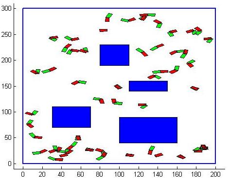
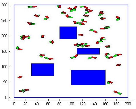
Considering the collision checks made in each sampling step, the resulting samples have the following properties. The samples are all collision free, both with respect to obstacles and the boundary box. There is at least one edge between any two nodes which guarantees that there is no isolated nodes.The number of samples created is an important parameter to effect the result of the PRM' algorithm, thus; its change will be investigated in the Experiments heading. Following is a figure which shows the resulting samples created in a 2D world with a number of obstacles.
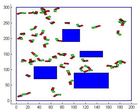
Figure 3.3.2 - Local Planner results, with a total of 50 samples created obeying the rules defined above. The red-green body blocks are the robots in their collision free configurations
In this step of the construction phase, the nodes generated in the local planner part are taken as inputs. These inputs are used to find the possible edges between any nodes to create a resulting unidirected graph. It is mentioned in the local planner that there is at least one edge between any two nodes among the samples. The roadmap construction step looks for more edges between the nodes.
In this part, each node is compared with every other node in the nodes list. Then the convex hull formed in the possible transition from these selected nodes are controlled for collision. If there is no collision, these nodes are added to the candidate neighboor nodes list. The idea of creating another candidate neighboor node list is to decrease the number of edges in order to speed up the graph based search algorithm which will be explained later on.
In each step, a candidate neighboor nodes list is created for the current node selected. In order to find the best of these neighboors, the nodes are sorted with respect to the path lengths. I have used the Euclidian distance between the base points of the two nodes' robots. An important parameter which will effect the result of the PRM' algorithm is the number of neighboor nodes which will be linked to the selected node.
The roadmap planner returns a unidirected graph which will be used as an input for the graph based search algorithm. Following is the result of the roadmap planner.
 |
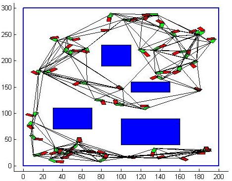 |
Figure 3.3.3 - Figure on the left shows the result of the local planner and the figure on the right is the resulting roadmap generated upon the nodes. The black lines represent the selected neighbooring edges
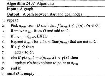
Query phase is the step where any graph based search algorithm could be used to find the shortest path from the start state to the goal state. I have preferred to use the A* Search algorithm which was used in the previous assignment. A* Search will return the shortest path or it will return failure case if there is no connection between the start and goal states. I am pasting the A* Search algorithm details from the previous assignment.
A* search is a best first graph based search algorithm that finds the shortest path between two nodes in the graph. An important function used in this search algorithm is a heuristic information that leads the search towards the goal. This heuristic information is an estimate about the distance to the goal in our case. Where many data could be used as heuristics, in visibility graph approach the Euclidian distance between the current node and the goal is preferred.
The search algorithm starts with an initial number of nodes that are neighboor to the starting point. In each iteration algorithm looks for the value of a function f(n) = g(n) + h(n) for each node n. This value is the sum heuristic about the distance to the goal and the real distance covered so far in order to reach that node. For each node with a value of function f(n), the algorithm selects the node with this minimum value and expands the neighboors of this selected node n. During the process, any node which has the minimum value of f(n) is selected.
A* search also remembers the nodes visited in each iteration. This memory both avoids the re-visiting of nodes and is used for back tracking when the shortest path is found between the start and goal nodes. With the notations given, the A* search algorithm is as below.
O = Open set, or priority queue which includes the nodes that are subject to search at an iteration step
C = Closed set, the visited nodes so far
c(n1,n2) = the length of the edge connecting n1 and n2
g(n) = total length covered so far in order to reach node n
h(n) = heuristic cost function, or the Euclidian distance from node n to goal
f(n) = g(n) + h(n) main criteria for search and selection evaluation
 |
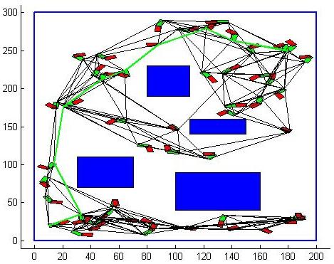 |
Figure 3.4.1 - The algorithm shows the A* Search. The figure on the right shows the shortest path from the start state and the goal state according to the A*Search. This shortest path is shown with thick green line.
I have used MATLAB to implement the customized PRM' algorithm. The random generator used in probabilistic local planner is the default MATLAB rand() function. I have not used an external specific collision checker, for this purpose I have used MATLAB's polybool() function for polygon intersection and union results which I have compared with the robot and obstacles to control collision. The source code for the whole implementation could be found here.
There are some important parameters which really effect the result of the PRM' algorithm. Those are; the total number of samples generated and the number of neighboors to connect to each node. The effect of the number of transition states during convex hull check and the random sampling is not invastigated in experiments but are discussed in the Observations heading.
For the experiments, I have set up XXX different environments. The first environment is a comparably less obstacle including workspace which will show the running time of the PRM' algorithm with fixed parameters for number of states and the number of neighboors. The second experiment will include more obstacles than the first one and will show the increase of time required to find collision free nodes and edges to solve the problem. Again, the same parameters used in the first experiment will be used here. The last experiment will have a specially built obstacle which will be a narrow passage. The aim of this experiment is to change parameters to check the result of the PRM' algorithm.
In this experiment the start state is qstart = [10 20 0.2 0.5] and qend = [180 250 1 1.2] for the robot. There are 4 polygonal obstacles in the workspace. The fixed parameters are as followed: number of states = 50, the neighboor count = 4. Here are the graphical results followed by the analytical results.
 |
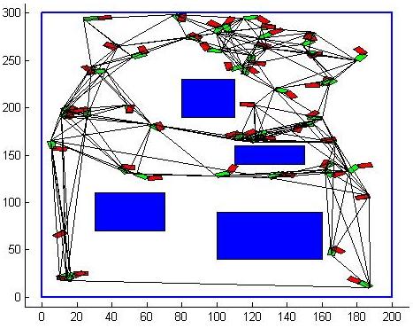 |
Figure 5.1 - The figure on the left shows the samples. The figure on the right shows the roadmap generated
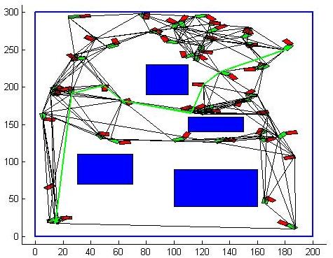
Figure 5.2 - Green thick line shows the A* Search result
Local Planner |
RoadMap Construction |
A* Search |
Total |
4,659767 secs |
26,740452 secs |
1,374788 secs |
32,775007 secs |
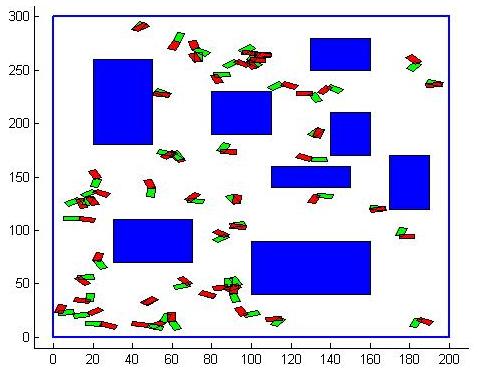
In this experiment the start state is qstart = [10 20 0.2 0.5] and qend = [180 250 1 1.2] for the robot. There are 8 polygonal obstacles in the workspace. The fixed parameters are as followed: number of states = 50, the neighboor count = 4. Here are the graphical results followed by the analytical results.
 |
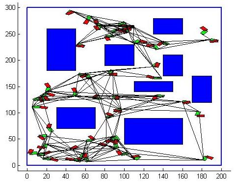 |
Figure 5.3 - The figures above the resulting samples and the roadmap generated. Reader may notice that, the samples in this experiment are densely found in the collision free spaces which are smaller regions compared to the previous experiment.
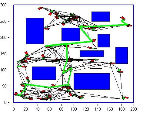
Figure 5.4 - The resulting path constructed. Notice the bug in the A* Search
Local Planner |
RoadMap Construction |
A* Search |
Total |
16,520641 secs |
47,848083 secs |
10,082988 secs |
74,451712 secs |
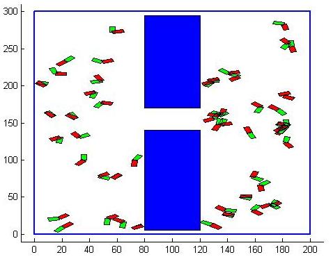
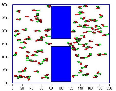
In this experiment the start state is qstart = [10 20 0.2 0.5] and qend = [180 250 1 1.2] for the robot. There are only 2 polygon obstacles in the workspace but the form a narrow passage which will harden the problem. The fixed parameters are as followed: number of states = 50, the neighboor count = 4. Here are the graphical results followed by the analytical results.
 |
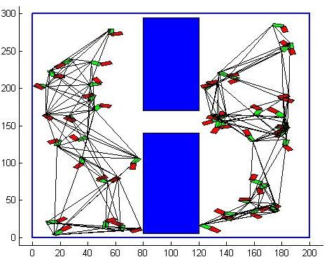 |
Figure 5.5 - The figure on the left shows the narrow passage built intentionally to harden the PRM' solution. Samples are nearly equally distributed by the sampler. The roadmap on the right shows two distinct unidirected graphs.
Although the sampler produces nearly equally distributed samples on both sides of the passage, the roadmap constructor could not find any possible connection between the nodes. As there is no possible way to reach from start state to the goal state the A* Search returns the fail case and reports unsuccessful solution.In the next experiment the parameters will be changed to increase the chance of finding a possible solution for this kind of problem. However it should be noted that, it is possible for PRM' to solve this problem with the given parameters. I have intentionally did not show the successful solution for this case.
Local Planner |
RoadMap Construction |
A* Search |
Total |
2,645356 secs |
16,663318 secs |
- |
- |
In this experiment the start state is qstart = [10 20 0.2 0.5] and qend = [180 250 1 1.2] for the robot. The map confiiguration is the same as the previous experiment. But this time the fixed parameters are changed: number of states = 100, the neighboor count = 6. Here are the graphical results followed by the analytical results.
 |
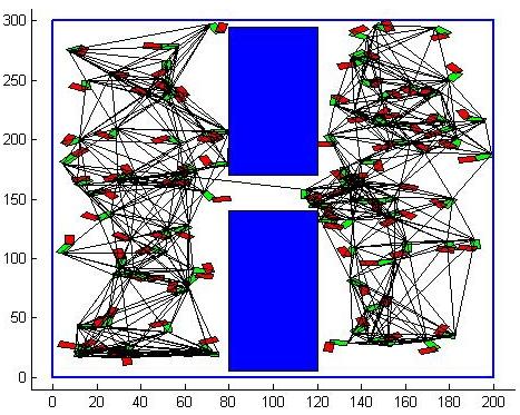 |
Figure 5.6 - Increased number of samples are shown on the left figure. The figure on the right shows that roadmap constructor could find a single path between the graphs on either side of the passage.
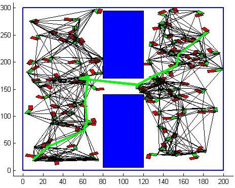
Figure 5.7 - The resulting path from start state to goal state
Increasing the number of samples and the neighboor nodes seems to solve the problem. But it should be stressed that, as this is a sampling based probabilistic approach, it cannot be said that increasing these parameters will surely solve the problem. I have observed cases where this parameter configuration did not solve this problem case. On the other hand, the previous case was once solved with the previous parameter set.
However it can be said that, increasing the number of nodes in the graph increases the probability of solving the problem.
Local Planner |
RoadMap Construction |
A* Search |
Total |
6,285572 secs |
65,758363 secs |
31,391722 secs |
103,435657 secs |
As mentioned before, the local sampler has been selected independent from node locations. Before this decision, each new node was sampled with respect to the position and orientation of the previous node. Therefore the possible pose of the new robot was stricted to fit in a small region around the previous node. In order to increase the free sample location possibilities the random sampler has been switched to become independent of other node location and orientations.
It is mentioned that the convex hull checker generates a number of transition states between the two nodes which are investigated for possible egde formation. In my experiments above, the number for transition states was 20. Changing this number would not effect the overall algorithm if the overall map is small and obstacles are not so complex polygons.
However if the map is large and there are complex shaped obstacles increasing the transition states would result in a more realistic convex hull. But this change will increase the computation time too.
[1] "Principles of Robot Motion" by Choset H. et.al. Ch:7 Pg: 202-225
[2] "MATLAB rand() Function" http://www.mathworks.com/access/helpdesk_r13/help/techdoc/ref/rand.html
[3] "Mersenne Twister Home Page" http://www.math.sci.hiroshima-u.ac.jp/~m-mat/MT/emt.html
[4] "Mersenne Twister Algorithm" Wikipedia, http://en.wikipedia.org/wiki/Mersenne_twister
[5] "MATLAB polybool() Function" http://www.mathworks.com/access/helpdesk/help/toolbox/map/ref/polybool.html
[6] "Convex Hull" Wikipedia, http://en.wikipedia.org/wiki/Convex_hull
Utku Çulha - Bilkent University
Computer Engineering Department